

Linear Regression
Mastering Predictive Analytics with R 의 내용을 기본으로 하여 일부 코드를 수정하거나 추가했다.
해당 책의 Chapter2 : Linear Regression을 바탕으로 작성했다.
Data
caret 패키지의 cars 데이터를 data_envir의 하위 항목으로 로드한다
Kelly Blue Book resale data for 2005 model year GM cars
R이 기본적으로 cars 데이터를 로드한 상태이기 때문에 caret의 cars를 불러오면 데이터를 덮어쓰게 된다. 덮어쓰는 것이 상관없다면 caret 패키지를 불러온 다음에 그냥 data(cars)를 실행시키면 된다
library(caret)
data(cars)
덮어쓰지 않고 다른 변수에 데이터를 불러오려면 아래와 같이 할 수 있다
우선, 비어있는 environment를 생성한다
data_envir = new.env(parent = .GlobalEnv)
ls 함수를 통해 해당 environment는 비어있음을 확인할 수 있다
ls(data_envir)
## character(0)
caret 패키지에서 cars데이터를 불러와서 data_envir에 저장한다
library(caret)

data(cars, package = 'caret', envir = data_envir)
ls(data_envir)
## [1] "cars"
list와 비슷한 방식으로 불러올 수 있다
head(data_envir$cars)
##      Price Mileage Cylinder Doors Cruise Sound Leather Buick Cadillac
## 1 22661.05   20105        6     4      1     0       0     1        0
## 2 21725.01   13457        6     2      1     1       0     0        0
## 3 29142.71   31655        4     2      1     1       1     0        0
## 4 30731.94   22479        4     2      1     0       0     0        0
## 5 33358.77   17590        4     2      1     1       1     0        0
## 6 30315.17   23635        4     2      1     0       0     0        0
##   Chevy Pontiac Saab Saturn convertible coupe hatchback sedan wagon
## 1     0       0    0      0           0     0         0     1     0
## 2     1       0    0      0           0     1         0     0     0
## 3     0       0    1      0           1     0         0     0     0
## 4     0       0    1      0           1     0         0     0     0
## 5     0       0    1      0           1     0         0     0     0
## 6     0       0    1      0           1     0         0     0     0
변수간의 상관관계를 확인하기 위해서 cor 함수로 correlation matrix를 생성한다
findCorrelation 함수를 통해 correlation이 높아서 제거해야할 열이 있는지 확인할 수 있다
cars_cor = cor(data_envir$cars)
findCorrelation(cars_cor)
## integer(0)
cutoff를 임의로 변경해서 확인할 수 있다. 기본값보다 높은 기준치를 부여했다.
findCorrelation(cars_cor, cutoff = 0.75)
## [1] 4
names(data_envir$cars)[4]
## [1] "Doors"
Doors 변수가 correlation이 높은 변수로 선정되었다.
차량이 coupe일 경우 문은 2개일 수밖에 없다. 따라서 Doors와 coupe 변수는 높은 상관관계를 가진다
with(data_envir$cars, cor(Doors, coupe))
## [1] -0.8254435
with(data_envir$cars, table(Doors, coupe))
##      coupe
## Doors   0   1
##     2  50 140
##     4 614   0
sedan 변수도 마찬가지다
with(data_envir$cars, cor(Doors, sedan))
## [1] 0.6949056
with(data_envir$cars, table(Doors, sedan))
##      sedan
## Doors   0   1
##     2 190   0
##     4 124 490
변수간의 linear dependency를 해결하기 위해서는 findLinearCombos 함수를 사용한다
findLinearCombos(data_envir$cars)
## $linearCombos
## $linearCombos[[1]]
## [1] 15  4  8  9 10 11 12 13 14
##
## $linearCombos[[2]]
##  [1] 18  4  8  9 10 11 12 13 16 17
##
##
## $remove
## [1] 15 18
결과는 list 형태가 된다
$linearCombos 에는 linear combination이 존재할 때 서로 의존관계에 있는 변수들의 column index가 나열된다
$remove는 linear combination을 없애기 위해서 제거해야할 열의 index를 보여준다
제거해야할 열만 idx_remove 벡터에 저장한다
idx_remove = findLinearCombos(data_envir$cars)$remove
cars_trim = data_envir$cars[, - idx_remove]
caret의 createDataPartition 함수를 통해서 training set과 test set을 분리시킨다.
동일한 결과물을 보기 위해서 random seed를 특정 값으로 고정시킨다. 해당 함수를 통해서 training set의 row index를 생성하고 traing set과 test set을 각각 분리한다
set.seed(123)
idx_cars_tr = createDataPartition(cars_trim$Price, p = 0.85, list = FALSE)
cars_tr = cars_trim[idx_cars_tr, ]
cars_ts = cars_trim[-idx_cars_tr, ]
Linear Model
가장 기본적인 linear model을 생성한다
종속변수는 Price
독립변수는 .으로 두면 나머지 모든 변수를 지정한다
summary 함수를 통해 model의 기본적인 내용을 살펴볼 수 있다
lm_cars = lm(Price ~ ., data = cars_tr)
summary(lm_cars)
##
## Call:
## lm(formula = Price ~ ., data = cars_tr)
##
## Residuals:
##     Min      1Q  Median      3Q     Max
## -9672.9 -1556.3   221.8  1468.6 13259.7
##
## Coefficients: (1 not defined because of singularities)
##               Estimate Std. Error t value Pr(>|t|)
## (Intercept) -9.962e+02  1.100e+03  -0.906  0.36524
## Mileage     -1.791e-01  1.388e-02 -12.901  < 2e-16 ***
## Cylinder     3.555e+03  1.249e+02  28.472  < 2e-16 ***
## Doors        1.631e+03  2.838e+02   5.745 1.39e-08 ***
## Cruise       4.131e+02  3.213e+02   1.285  0.19907
## Sound        5.480e+02  2.548e+02   2.150  0.03189 *
## Leather      7.012e+02  2.687e+02   2.609  0.00928 **
## Buick        1.124e+03  5.956e+02   1.887  0.05956 .
## Cadillac     1.381e+04  6.785e+02  20.355  < 2e-16 ***
## Chevy       -5.660e+02  4.642e+02  -1.219  0.22316
## Pontiac     -1.309e+03  5.187e+02  -2.524  0.01184 *
## Saab         1.204e+04  5.914e+02  20.353  < 2e-16 ***
## Saturn              NA         NA      NA       NA
## convertible  1.142e+04  5.942e+02  19.219  < 2e-16 ***
## hatchback   -6.286e+03  6.683e+02  -9.407  < 2e-16 ***
## sedan       -4.494e+03  4.828e+02  -9.308  < 2e-16 ***
## ---
## Signif. codes:  0 '***' 0.001 '**' 0.01 '*' 0.05 '.' 0.1 ' ' 1
##
## Residual standard error: 2924 on 669 degrees of freedom
## Multiple R-squared:  0.9172,	Adjusted R-squared:  0.9155
## F-statistic: 529.5 on 14 and 669 DF,  p-value: < 2.2e-16
1 not defined because of singularities 로 인해서 coeffiecient를 구할 수 없다고 나온다. linear dependency를 발생시키는 변수를 찾아서 제거해야 한다. alias 함수를 통해 살펴볼 수 있다
alias(lm_cars)
## Model :
## Price ~ Mileage + Cylinder + Doors + Cruise + Sound + Leather +
##     Buick + Cadillac + Chevy + Pontiac + Saab + Saturn + convertible +
##     hatchback + sedan
##
## Complete :
##        (Intercept) Mileage Cylinder Doors Cruise Sound Leather Buick
## Saturn  1           0       0        0     0      0     0      -1
##        Cadillac Chevy Pontiac Saab convertible hatchback sedan
## Saturn -1       -1    -1      -1    0           0         0
문제가 되는 변수는 Saturn이라는 것을 알 수 있다. Saturn 변수를 제거하고 다시 모델을 구성한다. 변수명 앞에 -를 입력하면 해당 변수를 제외하고 모델을 생성한다
lm_cars2 = lm(Price ~ . -Saturn, data = cars_tr)
summary(lm_cars2)
##
## Call:
## lm(formula = Price ~ . - Saturn, data = cars_tr)
##
## Residuals:
##     Min      1Q  Median      3Q     Max
## -9672.9 -1556.3   221.8  1468.6 13259.7
##
## Coefficients:
##               Estimate Std. Error t value Pr(>|t|)
## (Intercept) -9.962e+02  1.100e+03  -0.906  0.36524
## Mileage     -1.791e-01  1.388e-02 -12.901  < 2e-16 ***
## Cylinder     3.555e+03  1.249e+02  28.472  < 2e-16 ***
## Doors        1.631e+03  2.838e+02   5.745 1.39e-08 ***
## Cruise       4.131e+02  3.213e+02   1.285  0.19907
## Sound        5.480e+02  2.548e+02   2.150  0.03189 *
## Leather      7.012e+02  2.687e+02   2.609  0.00928 **
## Buick        1.124e+03  5.956e+02   1.887  0.05956 .
## Cadillac     1.381e+04  6.785e+02  20.355  < 2e-16 ***
## Chevy       -5.660e+02  4.642e+02  -1.219  0.22316
## Pontiac     -1.309e+03  5.187e+02  -2.524  0.01184 *
## Saab         1.204e+04  5.914e+02  20.353  < 2e-16 ***
## convertible  1.142e+04  5.942e+02  19.219  < 2e-16 ***
## hatchback   -6.286e+03  6.683e+02  -9.407  < 2e-16 ***
## sedan       -4.494e+03  4.828e+02  -9.308  < 2e-16 ***
## ---
## Signif. codes:  0 '***' 0.001 '**' 0.01 '*' 0.05 '.' 0.1 ' ' 1
##
## Residual standard error: 2924 on 669 degrees of freedom
## Multiple R-squared:  0.9172,	Adjusted R-squared:  0.9155
## F-statistic: 529.5 on 14 and 669 DF,  p-value: < 2.2e-16
Residual
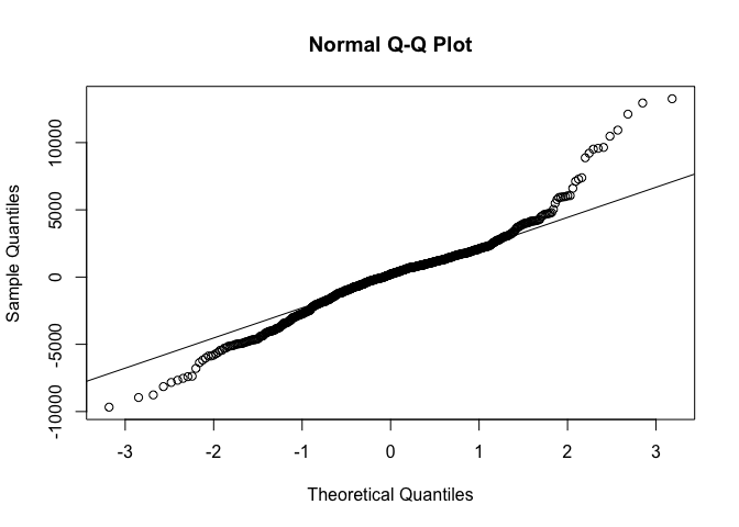
residual(잔차)이 정규분포를 따르는지 확인하기 위해서 qqnorm, qqline 함수로 차트를 그려볼 수 있다
qqnorm(lm_cars2$residuals)
qqline(lm_cars2$residuals)
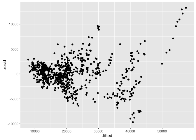
residual plot with ggplot2
ggplot2의 fortify 함수를 사용하면 lm 객체를 data.frame 형식으로 바로 변경할 수 있다. 모형의 잔차를 그래프로 나타내려고 한다.
library(ggplot2)
head(fortify(lm_cars2))
##      Price Mileage Cylinder Doors Cruise Sound Leather Buick Cadillac
## 1 22661.05   20105        6     4      1     0       0     1        0
## 3 29142.71   31655        4     2      1     1       1     0        0
## 5 33358.77   17590        4     2      1     1       1     0        0
## 6 30315.17   23635        4     2      1     0       0     0        0
## 7 33381.82   17381        4     2      1     1       1     0        0
## 8 30251.02   27558        4     2      1     0       1     0        0
##   Chevy Pontiac Saab Saturn convertible hatchback sedan       .hat
## 1     0       0    0      0           0         0     1 0.01921885
## 3     0       0    1      0           1         0     0 0.03090775
## 5     0       0    1      0           1         0     0 0.02872264
## 6     0       0    1      0           1         0     0 0.03368733
## 7     0       0    1      0           1         0     0 0.02875741
## 8     0       0    1      0           1         0     0 0.03270262
##     .sigma      .cooksd  .fitted    .resid  .stdresid
## 1 2925.202 0.0008680549 20300.17  2360.883  0.8151576
## 3 2914.451 0.0118389976 35936.02 -6793.309 -2.3596737
## 5 2919.808 0.0061645819 38455.31 -5096.539 -1.7683038
## 6 2917.714 0.0094868754 36123.33 -5808.159 -2.0203787
## 7 2919.769 0.0062073810 38492.74 -5110.925 -1.7733268
## 8 2917.529 0.0093902378 36121.85 -5870.830 -2.0411393
ggplot(fortify(lm_cars2), aes(x = .fitted, y = .resid))+
  geom_point()
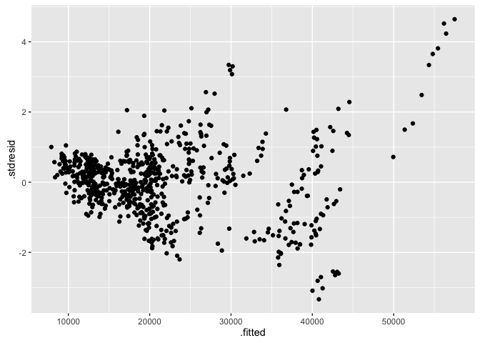
표준화된 residual은 .stdresid 변수를 사용한다. y축이 변경되는 것을 볼 수 있다.
ggplot(fortify(lm_cars2), aes(x = .fitted, y = .stdresid))+
  geom_point()
Shapiro-Wilk Normality Test
Shapiro-Wilk의 정규성 테스트를 해볼 수 있다
shapiro.test(lm_cars2$residuals)
##
## 	Shapiro-Wilk normality test
##
## data:  lm_cars2$residuals
## W = 0.9595, p-value = 8.544e-13
ANOVA table
anova 함수를 사용하면 하나 이상의 model객체를 통해서 ANOVA table을 생성할 수 있다. 여기서는 intercept의 존재만 가정하는 Null Model을 생성한 다음에. 위에서 생성했던 model과 비교한다. 변수들이 실제로 효과가 있는지 없는지의 여부를 테스트할 수 있다
lm_cars_null = lm(Price ~ 1, data = cars_tr)
anova(lm_cars2, lm_cars_null)
## Analysis of Variance Table
##
## Model 1: Price ~ (Mileage + Cylinder + Doors + Cruise + Sound + Leather +
##     Buick + Cadillac + Chevy + Pontiac + Saab + Saturn + convertible +
##     hatchback + sedan) - Saturn
## Model 2: Price ~ 1
##   Res.Df        RSS  Df   Sum of Sq      F    Pr(>F)
## 1    669 5.7216e+09
## 2    683 6.9127e+10 -14 -6.3405e+10 529.55 < 2.2e-16 ***
## ---
## Signif. codes:  0 '***' 0.001 '**' 0.01 '*' 0.05 '.' 0.1 ' ' 1
p-value가 0에 가깝다는 것을 확인할 수 있다
Performance metric
모델의 성능을 평가하는 방법은 여러 가지가 있다. 여기서는 가장 간단하고 살펴볼 수 있는 R-squared를 살펴본다. R-squared와 값이 일부 조정된 Adjusted R-squared는 summary 함수의 결과물에서 볼 수 있다
summary_cars2 = summary(lm_cars2)

summary_cars2$r.squared
## [1] 0.91723
summary_cars2$adj.r.squared
## [1] 0.9154979
R-squared는 평균을 기준으로 데이터 전체의 변동량에서 실제값과 예측값의 차이가 얼마나 비슷한지를 알려준다. 실제값과 예측값이 정확이 같다면 1이된다
실제로 R-squared를 구하는 과정을 살펴보면 아래와 같다
ssr_cars = sum((lm_cars$fitted.values - cars_tr$Price)^2)
sst_cars = sum((cars_tr$Price - mean(cars_tr$Price))^2)
r2_cars = 1 - ssr_cars / sst_cars
r2_cars
## [1] 0.91723
결과물은 위에서 구한 R-Squared와 같다
R-Squared는 단순하면서도 직관적이라는 장점이 있다. 하지만 의미없는 변수를 추가하더라도 값이 계속 증가한다는 단점이 있다. 따라서 이러한 문제를 보완하기 위한 Adjusted R-Squared는 feature의 개수를 통해 값을 보정한다
n_cars = nrow(cars_tr)
k_cars = length(lm_cars2$coefficients) - 1 # intercept를 제외한 feature의 개수
ar2_cars = 1 - (1 - r2_cars) * (n_cars - 1) / (n_cars - k_cars - 1)
ar2_cars
## [1] 0.9154979
Test set Performance
predict 함수를 통해 model을 가지고 test set의 결과물을 예측한다
pred_cars2 = predict(lm_cars2, cars_ts[-1])
실제값과 예측값의 차이를 통해 모델이 실제와 얼마나 차이가 있는지 값을 측정할 수 있다
mse_cars2 = mean((pred_cars2 - cars_ts$Price)^2)
mse_cars2
## [1] 8019592
실제 데이터와 예측 결과를 하나의 그래프에 표현하려고 한다
library(dplyr)

diff_cars2 = data.frame(
    price = cars_ts$Price,
    pred = pred_cars2) %>%
  arrange(price) %>%
  mutate(idx = row_number())
ggplot2에서 본래 추구하는 방식으로 그래프를 그리기 위해서는 tidy data의 형태로 data.frame을 정리하는 것이 좋다. tidy data에 대해서 알아보려면 예전 글 의 내용을 참고하면 좋을 것 같다.
diff_cars2_tidy = diff_cars2 %>%
  tidyr::gather(key = "level", value = "value", price:pred)

head(diff_cars2_tidy)
##   idx level    value
## 1   1 price  8638.93
## 2   2 price  9789.04
## 3   3 price 10354.04
## 4   4 price 10813.34
## 5   5 price 10921.95
## 6   6 price 11343.05
ggplot(data = diff_cars2_tidy,
        aes(x = idx, y = value, colour = level)) +
  geom_point()

Feature Selection
step 함수를 통해서 backward selection을 시행한다. 모든 요소를 포함한 상태에서 모델을 생성하고, 설명력이 떨어지는 변수를 제거하면서 더 나은 모델을 찾아나가는 방식이다. 결과물에서는 AIC가 낮을 수록 좋은 model이다
lm_cars3 = step(lm_cars2,
                scope = list(lower = lm_cars_null, upper = lm_cars2),
                direction = 'backward')
## Start:  AIC=10932.66
## Price ~ (Mileage + Cylinder + Doors + Cruise + Sound + Leather +
##     Buick + Cadillac + Chevy + Pontiac + Saab + Saturn + convertible +
##     hatchback + sedan) - Saturn
##
##               Df  Sum of Sq        RSS   AIC
## - Chevy        1   12714941 5.7343e+09 10932
## - Cruise       1   14132676 5.7358e+09 10932
## <none>                      5.7216e+09 10933
## - Buick        1   30460987 5.7521e+09 10934
## - Sound        1   39546468 5.7612e+09 10935
## - Pontiac      1   54481904 5.7761e+09 10937
## - Leather      1   58221312 5.7799e+09 10938
## - Doors        1  282297010 6.0039e+09 10964
## - sedan        1  741046049 6.4627e+09 11014
## - hatchback    1  756759889 6.4784e+09 11016
## - Mileage      1 1423416473 7.1450e+09 11083
## - convertible  1 3159154955 8.8808e+09 11231
## - Saab         1 3542704945 9.2643e+09 11260
## - Cadillac     1 3543395686 9.2650e+09 11260
## - Cylinder     1 6933034432 1.2655e+10 11474
##
## Step:  AIC=10932.18
## Price ~ Mileage + Cylinder + Doors + Cruise + Sound + Leather +
##     Buick + Cadillac + Pontiac + Saab + convertible + hatchback +
##     sedan
##
##               Df  Sum of Sq        RSS   AIC
## - Cruise       1   11655088 5.7460e+09 10932
## <none>                      5.7343e+09 10932
## - Sound        1   32601330 5.7669e+09 10934
## - Pontiac      1   49199044 5.7835e+09 10936
## - Leather      1   51468366 5.7858e+09 10936
## - Buick        1  106476733 5.8408e+09 10943
## - Doors        1  273386852 6.0077e+09 10962
## - sedan        1  730783107 6.4651e+09 11012
## - hatchback    1  777551120 6.5119e+09 11017
## - Mileage      1 1421303710 7.1556e+09 11082
## - convertible  1 3147012333 8.8814e+09 11229
## - Cadillac     1 6406507443 1.2141e+10 11443
## - Saab         1 6436594114 1.2171e+10 11445
## - Cylinder     1 6972320144 1.2707e+10 11474
##
## Step:  AIC=10931.57
## Price ~ Mileage + Cylinder + Doors + Sound + Leather + Buick +
##     Cadillac + Pontiac + Saab + convertible + hatchback + sedan
##
##               Df  Sum of Sq        RSS   AIC
## <none>                      5.7460e+09 10932
## - Sound        1   32581443 5.7786e+09 10933
## - Pontiac      1   46537556 5.7925e+09 10935
## - Leather      1   48481038 5.7945e+09 10935
## - Buick        1  122937808 5.8689e+09 10944
## - Doors        1  263004964 6.0090e+09 10960
## - sedan        1  719958937 6.4660e+09 11010
## - hatchback    1  789129020 6.5351e+09 11018
## - Mileage      1 1419476570 7.1655e+09 11081
## - convertible  1 3136917995 8.8829e+09 11228
## - Cadillac     1 6450570826 1.2197e+10 11444
## - Saab         1 7963463390 1.3709e+10 11524
## - Cylinder     1 8082905852 1.3829e+10 11530
summary(lm_cars3)
##
## Call:
## lm(formula = Price ~ Mileage + Cylinder + Doors + Sound + Leather +
##     Buick + Cadillac + Pontiac + Saab + convertible + hatchback +
##     sedan, data = cars_tr)
##
## Residuals:
##     Min      1Q  Median      3Q     Max
## -9664.4 -1598.7   199.8  1523.0 13304.8
##
## Coefficients:
##               Estimate Std. Error t value Pr(>|t|)
## (Intercept) -1.036e+03  1.086e+03  -0.953 0.340773
## Mileage     -1.789e-01  1.389e-02 -12.875  < 2e-16 ***
## Cylinder     3.584e+03  1.167e+02  30.723  < 2e-16 ***
## Doors        1.551e+03  2.799e+02   5.542  4.3e-08 ***
## Sound        4.881e+02  2.503e+02   1.951 0.051523 .
## Leather      6.311e+02  2.653e+02   2.379 0.017620 *
## Buick        1.689e+03  4.457e+02   3.789 0.000165 ***
## Cadillac     1.437e+04  5.235e+02  27.446  < 2e-16 ***
## Pontiac     -8.204e+02  3.519e+02  -2.331 0.020038 *
## Saab         1.271e+04  4.169e+02  30.495  < 2e-16 ***
## convertible  1.133e+04  5.918e+02  19.139  < 2e-16 ***
## hatchback   -6.391e+03  6.657e+02  -9.600  < 2e-16 ***
## sedan       -4.399e+03  4.797e+02  -9.169  < 2e-16 ***
## ---
## Signif. codes:  0 '***' 0.001 '**' 0.01 '*' 0.05 '.' 0.1 ' ' 1
##
## Residual standard error: 2926 on 671 degrees of freedom
## Multiple R-squared:  0.9169,	Adjusted R-squared:  0.9154
## F-statistic: 616.8 on 12 and 671 DF,  p-value: < 2.2e-16
step 함수를 사용하면 현재 상황에서 각 변수를 빼거나 추가했을 때 AIC가 어떻게 변화하는지 파악한다. 만약 현재의 모델이 가장 낮은 AIC를 나타낸다면 해당 모델로 최종 확정하게 된다. 변수를 비교하는 방식은 forward, backward, 그리고 양쪽을 모두 사용하는 both 등 다양한 방식을 지원한다.
lm_cars4 = step(lm_cars2,
                scope = list(lower = lm_cars_null, upper = lm_cars2),
                direction = 'both')
## Start:  AIC=10932.66
## Price ~ (Mileage + Cylinder + Doors + Cruise + Sound + Leather +
##     Buick + Cadillac + Chevy + Pontiac + Saab + Saturn + convertible +
##     hatchback + sedan) - Saturn
##
##               Df  Sum of Sq        RSS   AIC
## - Chevy        1   12714941 5.7343e+09 10932
## - Cruise       1   14132676 5.7358e+09 10932
## <none>                      5.7216e+09 10933
## - Buick        1   30460987 5.7521e+09 10934
## - Sound        1   39546468 5.7612e+09 10935
## - Pontiac      1   54481904 5.7761e+09 10937
## - Leather      1   58221312 5.7799e+09 10938
## - Doors        1  282297010 6.0039e+09 10964
## - sedan        1  741046049 6.4627e+09 11014
## - hatchback    1  756759889 6.4784e+09 11016
## - Mileage      1 1423416473 7.1450e+09 11083
## - convertible  1 3159154955 8.8808e+09 11231
## - Saab         1 3542704945 9.2643e+09 11260
## - Cadillac     1 3543395686 9.2650e+09 11260
## - Cylinder     1 6933034432 1.2655e+10 11474
##
## Step:  AIC=10932.18
## Price ~ Mileage + Cylinder + Doors + Cruise + Sound + Leather +
##     Buick + Cadillac + Pontiac + Saab + convertible + hatchback +
##     sedan
##
##               Df  Sum of Sq        RSS   AIC
## - Cruise       1   11655088 5.7460e+09 10932
## <none>                      5.7343e+09 10932
## + Chevy        1   12714941 5.7216e+09 10933
## - Sound        1   32601330 5.7669e+09 10934
## - Pontiac      1   49199044 5.7835e+09 10936
## - Leather      1   51468366 5.7858e+09 10936
## - Buick        1  106476733 5.8408e+09 10943
## - Doors        1  273386852 6.0077e+09 10962
## - sedan        1  730783107 6.4651e+09 11012
## - hatchback    1  777551120 6.5119e+09 11017
## - Mileage      1 1421303710 7.1556e+09 11082
## - convertible  1 3147012333 8.8814e+09 11229
## - Cadillac     1 6406507443 1.2141e+10 11443
## - Saab         1 6436594114 1.2171e+10 11445
## - Cylinder     1 6972320144 1.2707e+10 11474
##
## Step:  AIC=10931.57
## Price ~ Mileage + Cylinder + Doors + Sound + Leather + Buick +
##     Cadillac + Pontiac + Saab + convertible + hatchback + sedan
##
##               Df  Sum of Sq        RSS   AIC
## <none>                      5.7460e+09 10932
## + Cruise       1   11655088 5.7343e+09 10932
## + Chevy        1   10237353 5.7358e+09 10932
## - Sound        1   32581443 5.7786e+09 10933
## - Pontiac      1   46537556 5.7925e+09 10935
## - Leather      1   48481038 5.7945e+09 10935
## - Buick        1  122937808 5.8689e+09 10944
## - Doors        1  263004964 6.0090e+09 10960
## - sedan        1  719958937 6.4660e+09 11010
## - hatchback    1  789129020 6.5351e+09 11018
## - Mileage      1 1419476570 7.1655e+09 11081
## - convertible  1 3136917995 8.8829e+09 11228
## - Cadillac     1 6450570826 1.2197e+10 11444
## - Saab         1 7963463390 1.3709e+10 11524
## - Cylinder     1 8082905852 1.3829e+10 11530
summary(lm_cars4)
##
## Call:
## lm(formula = Price ~ Mileage + Cylinder + Doors + Sound + Leather +
##     Buick + Cadillac + Pontiac + Saab + convertible + hatchback +
##     sedan, data = cars_tr)
##
## Residuals:
##     Min      1Q  Median      3Q     Max
## -9664.4 -1598.7   199.8  1523.0 13304.8
##
## Coefficients:
##               Estimate Std. Error t value Pr(>|t|)
## (Intercept) -1.036e+03  1.086e+03  -0.953 0.340773
## Mileage     -1.789e-01  1.389e-02 -12.875  < 2e-16 ***
## Cylinder     3.584e+03  1.167e+02  30.723  < 2e-16 ***
## Doors        1.551e+03  2.799e+02   5.542  4.3e-08 ***
## Sound        4.881e+02  2.503e+02   1.951 0.051523 .
## Leather      6.311e+02  2.653e+02   2.379 0.017620 *
## Buick        1.689e+03  4.457e+02   3.789 0.000165 ***
## Cadillac     1.437e+04  5.235e+02  27.446  < 2e-16 ***
## Pontiac     -8.204e+02  3.519e+02  -2.331 0.020038 *
## Saab         1.271e+04  4.169e+02  30.495  < 2e-16 ***
## convertible  1.133e+04  5.918e+02  19.139  < 2e-16 ***
## hatchback   -6.391e+03  6.657e+02  -9.600  < 2e-16 ***
## sedan       -4.399e+03  4.797e+02  -9.169  < 2e-16 ***
## ---
## Signif. codes:  0 '***' 0.001 '**' 0.01 '*' 0.05 '.' 0.1 ' ' 1
##
## Residual standard error: 2926 on 671 degrees of freedom
## Multiple R-squared:  0.9169,	Adjusted R-squared:  0.9154
## F-statistic: 616.8 on 12 and 671 DF,  p-value: < 2.2e-16
Regularization
변수 선택은 종종 overfitting(과적합)에 대응하는 방법으로 사용할 수 있다. regularization을 통해 특정 coefficient가 과도하게 큰 값을 갖지 않도록 조정할 수 있다.
ridge regression과 lasso는 penalty term에서 차이가 발생한다. ridge regression은 가중치가 작게 주어지더라도 각 변수들의 영향력이 남아있다. 하지만 lasso의 경우 가중치가 작은 경우 아예 0으로 수렴하는 경우가 발생한다
ridge regression
glmnet 패키지의 glmnet 함수를 통해 ridge regression과 lasso를 시행하려고 한다
첫 번째 parameter로는 feature들로 구성된 matrix를 필요로 한다. model.matrix 함수를 통해 design matrix를 생성한다
# 1열의 intercept만 제거한다
mat_cars_tr = model.matrix(Price ~ . -Saturn, data = cars_tr)[, -1]
두 번째 parameter는 결과물 변수들(여기서는 Price)로 구성된 벡터다
세 번째 parameter인 alpha는 0일 때 ridge regression, 1일 때 lasso를 시행한다
네 번째 parameter는 lambda 벡터이다. 모델을 생성할 때 이 값이 포함된 수식을 최소화시키는 방향으로 계산된다. 좋은 model을 생성하기 위해서는 가장 좋은 결과물을 내는 lambda값을 찾아야 한다. lambda parameter는 사용자가 직접 lambda sequence를 지정할 때 사용한다. 보통은 nlambda와 lambda.min.ratio 값을 사용해서 구하게끔 되어있다. 두 값 모두 기본값이 지정되어있기 때문에(100, 0.0001) 명시하지 않을경우 기본값을 사용한다
library(glmnet)
## Loading required package: Matrix
## Loading required package: foreach
## Loaded glmnet 2.0-2
model_ridge = glmnet(
  mat_cars_tr,
  cars_tr$Price,
  alpha = 0,
  lambda = 10 ^ seq(8, -4, length = 250)
)
lambda값에 250개짜리 벡터를 지정했기 때문에 250개의 model이 생성된다
coef함수를 통해 특정 model의 coefficient값을 볼 수 있다
coef(model_ridge)[,100]
##   (Intercept)       Mileage      Cylinder         Doors        Cruise
##  6336.6474394    -0.1552561  2725.2328259   387.8009432  1688.3451952
##         Sound       Leather         Buick      Cadillac         Chevy
##   214.7119462  1166.1893897  -411.9407312 11612.9688672 -2443.3869902
##       Pontiac          Saab   convertible     hatchback         sedan
## -2156.4412870  8344.4367057 10665.7039500 -3146.6877319 -2065.8999174
coef(model_ridge)[,200]
##   (Intercept)       Mileage      Cylinder         Doors        Cruise
##  -995.9883276    -0.1791173  3555.2756739  1630.6235076   413.1057260
##         Sound       Leather         Buick      Cadillac         Chevy
##   548.0081003   701.2180650  1123.9153032 13809.8266390  -566.0737694
##       Pontiac          Saab   convertible     hatchback         sedan
## -1309.3151867 12036.8172063 11420.4701519 -6286.0530466 -4493.8744852
좋은 lambda값을 찾을 수 있도록 하기 위해 glmnet 패키지에서는 cv.glmnet 함수를 제공한다. 교차검증을 통해 MSE를 최소화시키는 lambda를 찾는다
ridge_lambda = cv.glmnet(
  mat_cars_tr,
  cars_tr$Price,
  alpha = 0)
predict 함수를 통해 model을 바탕으로 test set의 값을 예측한다
s 에는 lambda값이 들어간다. type의 값을 바꾸면 다양한 결과물을 볼 수 있다
type = "coefficient" 일 때는 다음과 같은 정보를 알 수 있다
predict(
  model_ridge,
  s = ridge_lambda$lambda.min,
  type = 'coefficient')
## 15 x 1 sparse Matrix of class "dgCMatrix"
##                         1
## (Intercept)  3424.8104154
## Mileage        -0.1677827
## Cylinder     3102.4637324
## Doors         828.4585393
## Cruise       1166.4418117
## Sound         375.2800236
## Leather       994.0758585
## Buick          33.4808904
## Cadillac    12483.2985848
## Chevy       -1876.6192799
## Pontiac     -1970.2776716
## Saab         9872.9328182
## convertible 11090.0424876
## hatchback   -4216.6057859
## sedan       -2924.2738801
예측 결과물을 보려면 test set에 대해서도 matrix형태로 구성해야한다. predict.glmnet함수의 newx에 test set의 matrix를 전달한다
mat_cars_ts = model.matrix(Price ~ . -Saturn, data = cars_ts)[, -1]

pred_ridge = predict(
  model_ridge,
  s = ridge_lambda$lambda.min,
  newx = mat_cars_ts,
  type = 'response'
)

mse_ridge = mean((pred_ridge - cars_ts$Price)^2)
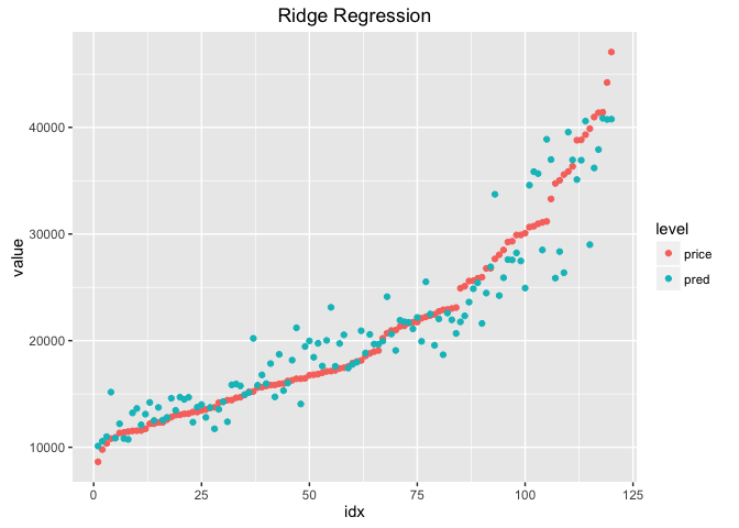
실제 값과 예측결과를 그래프로 비교해보려고 한다
df_ridge = data.frame(
    price = cars_ts$Price,
    pred = pred_ridge[,1]) %>%
  arrange(price) %>%
  mutate(idx = row_number()) %>%
  tidyr::gather(key = 'level', value = 'value', price:pred)

ggplot(df_ridge, aes(x = idx, y = value, colour = level))+
  geom_point()+
  ggtitle('Ridge Regression')
Lasso (Least Absolute Shrinkage and Selection Operator)
lasso는 ridge regression과 같은 방식으로 시행할 수 있다. alpha = 1로 설정하면 lasso가 동작한다
model_lasso = glmnet(
  mat_cars_tr,
  cars_tr$Price,
  alpha = 1,
  lambda = 10 ^ seq(8, -4, length = 250)
)

lasso_lambda = cv.glmnet(
  mat_cars_tr,
  cars_tr$Price,
  alpha = 1
)

pred_lasso = predict(
  model_lasso,
  s = lasso_lambda$lambda.min,
  newx = mat_cars_ts,
  type = 'response'
)

mse_lasso = mean((pred_lasso - cars_ts$Price)^2)
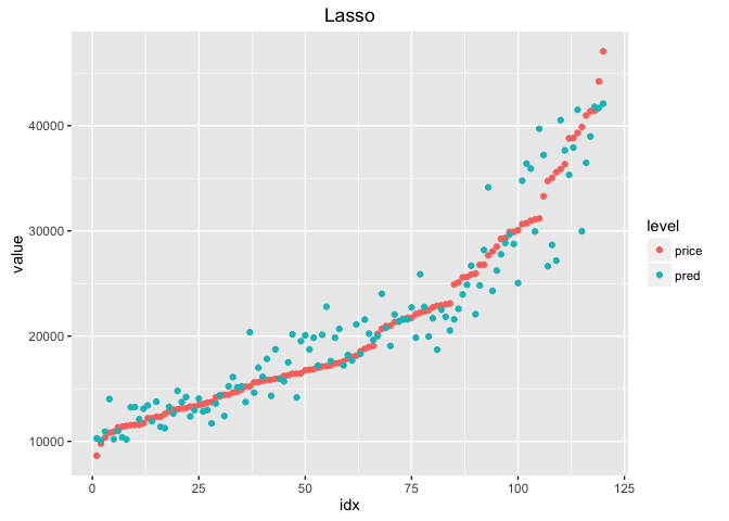
lasso의 경우도 실제 값과 예측결과를 그래프로 비교해볼 수 있다
df_lasso = data.frame(
    price = cars_ts$Price,
    pred = pred_lasso[,1]) %>%
  arrange(price) %>%
  mutate(idx = row_number()) %>%
  tidyr::gather(key = 'level', value = 'value', price:pred)

ggplot(df_lasso, aes(x = idx, y = value, colour = level))+
  geom_point()+
  ggtitle('Lasso')
각 모델의 MSE를 비교해보면 아래와 같다
mse_cars2 # mse of linear model
## [1] 8019592
mse_ridge # mse of ridge regression
## [1] 8661437
mse_lasso # mse of lasso
## [1] 8017329
위에서 lasso를 적용할 때는 이미 불필요한 변수를 제거한 상태였다 이번에는 변수를 제거하지 않은 상태에서 lasso를 적용해보려고 한다
cars_tr2 = data_envir$cars[idx_cars_tr, ]
cars_ts2 = data_envir$cars[-idx_cars_tr, ]

mat_cars_tr2 = model.matrix(Price ~ ., data = cars_tr2)[, -1]

model_lasso2 = glmnet(
  mat_cars_tr2,
  cars_tr2$Price,
  alpha = 1
)

lasso_lambda2 = cv.glmnet(
  mat_cars_tr2,
  cars_tr2$Price,
  alpha = 1
)

mat_cars_ts2 = model.matrix(Price ~ ., data = cars_ts2)[, -1]

pred_lasso2 = predict(
  model_lasso2,
  s = lasso_lambda2$lambda.min,
  newx = mat_cars_ts2
)

df_lasso2 = data.frame(
    price = cars_ts2$Price,
    pred = pred_lasso2[,1]) %>%
  arrange(price) %>%
  mutate(idx = row_number()) %>%
  tidyr::gather(key = 'level', value = 'value', price:pred)

ggplot(df_lasso2, aes(x = idx, y = value, colour = level))+
  geom_point()+
  ggtitle('Lasso2')

mse_lasso2 = mean((pred_lasso2 - cars_ts2$Price)^2)
mse_lasso2
## [1] 8037115
64번째 model을 살펴보면 Saturn, coupe, sedan의 coefficient가 0이라는 것을 볼 수 있다. 따라서 변수가 제거된 것과 같은 효과를 가진다.
coef(model_lasso2)[,64]
##  (Intercept)      Mileage     Cylinder        Doors       Cruise
##  3511.878810    -0.176481  3528.994492  -586.838372   412.692812
##        Sound      Leather        Buick     Cadillac        Chevy
##   488.060710   664.244892  1093.205029 13848.673141  -504.232147
##      Pontiac         Saab       Saturn  convertible        coupe
## -1204.322090 12028.003855     0.000000 11418.509547     0.000000
##    hatchback        sedan        wagon
## -1755.734835     0.000000  4352.276380